Oversimplified mathematical models and the so-called growth rate advantage
How risks of new SARS-CoV-2 variants are exaggerated in results from incomplete mathematical models

Mathematical models for the spread of new SARS-CoV-2 variants recently resulted in large growth rates comparable to that of the well-known variants of 2021. This led to what I find wrong conclusions about the dangers of new (sub)variants. The results were quickly communicated and shared on social media and sometimes so remarkable that they appeared in mainstream media outlets with headlines like variant of the “dog of hell”.1
The growth rates of variants since last winter appear for instance in charts like this:
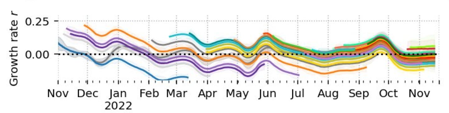
Here every line represents one variant and the r value is the daily growth rate. A variant that tops the bunch of lines means that it has the capability to replace previous variants. If the added growth rate is large, it will usually mean a surge of infections. This chain of events indeed has occurred previously with alpha, delta and omicron. Inspecting the above chart, it must be concluded that there are new subvariants Bx.x coming up every few months even in 2022 with similar aggressive "power" to start new waves as those historical variant-driven waves. Similar conclusion have also been drawn by other researchers and have spread on social media to be later amplified by media reports.
But actually I will argue that the above plot of growth curves is unrealistically static and even and really should be more skewed like this:
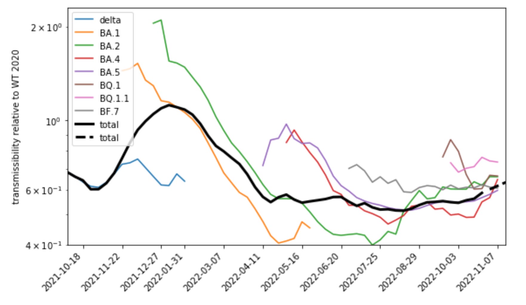
I will explain the meaning of the y-axis in this plot but for the moment take it as a rescaled growth rate. It can be clearly noted that the effects of more recent variants, e.g. BA.5 and BQ.1, are much smaller in this plot than that of the earlier variants including BA.1, the first omicron variant. In contrast to the first chart, the comparative advantage of the newer variants declines over the course of 2022 and is much smaller than that of the first omicron variant. Accordingly also the waves driven by these variants were smaller than initially expected.
Counting on contact numbers
The difference between the two approaches used above is that I have factored out the number of social contacts in the second plot. Since the beginning of the pandemic this number is approximately known from a large panel of cell-phone app users for Germany.2 For 2022 the number of social contacts per person and day did not stay constant but has increased from about 30 in January to more than 100 in September. This dynamics should be included in mathematical models, but, since it is essentially unknown for 99% of the world’s countries, this has not systematically been done so far. As far as I am aware of, this analysis for Germany is the only analysis where the contact numbers of a country’s population are known.
Since the projected growth rates and large waves did not come into being for instance in the case of BQ.1, we should reinspect the method used to derive the growth rates. Below I will analyse a frequently used simple model of reproduction numbers and growth rates and will identify what I suspect to be an important omission in the calculations. The problem — besides ignoring the unknown contact numbers — is the largely unknown distribution of generation times of SARS-CoV-2.
To understand this we have to dig a bit deeper into the mathematical relation of growth rates (i.e. the exponent of day-to-day exponential growth) and the reproduction number. The effective reproduction number is a measure of the average number of secondary cases produced by a single infected individual in a population and is defined by:
Here the right hand side is a product of the generation time, the number of contacts C per day, and the probability of a transmission given a contact (transmissibility). The generation time refers to the time it takes for an infected individual to infect another individual. For SARS-CoV-2 the mean of the generation time is usually estimated to 5 days (in most of the calculations for Germany, however, I will use the 4 days estimate chosen by Robert-Koch-Institut).
To compute R or — to evaluate the potential risk of a new variant — the different R values for variants, one often first determines the growth rates r for assumed exponential growths of the incidence numbers. There is an intuitive relation of r to R so that for R>1 the incidence grows and at the same time r should be larger than 0. Conversely, if a wave subsides, R<1 and we will find a negative “growth” rate r. Unfortunately, the exact relation between r and R is complex and depends in a nontrivial way not only on the mean but on the distribution of the generation time. This relation has been worked out in the past3 and, without going too much into the details, we will give two examples for this relation, and see how that affects the growth rate estimates.
From mean time to distributed times
The generation time of SARS-CoV-2 is not well-defined and may vary depending on the population and the specific circumstances of an outbreak. It is likely that the distribution is skewed towards shorter times, as transmission is more often to occur within a few days of symptom onset when the viral load is highest. However, there are cases of SARS-CoV-2 transmission occurring more than two weeks after symptom onset, indicating that there may be some individuals with longer generation times.
Nevertheless we will begin with a very basic distribution where each individual infects the next one after the exact same time. That means that we assume a delta distribution for the generation time and in this case the following relation of r and R is known to hold:
Here only the mean of the generation time enters. Next, if we consider two variants, for simplicity here called ‘wild type’ and ‘variant’, and divide the respective relations for r and R we get
With the definition of R given above we derive from this4:
Then we see that here the growth rate difference, or potential growth rate advantage, does not depend on the number of contacts. The value of C has dropped out and does not need to be known. Several authors have, possibly because of this reason, assumed the delta distribution that gets rid of the (unknown) contact number in the calculation.5
However, as mentioned above, the delta distribution is unrealistic and for more realistic distributions of the generation time, the growth rate advantage depends on contact numbers. For example, for an exponential distribution of the generation time we look up that
and then for the two variants we find:
In this case the growth rate difference depends on contacts. If a new and more transmissible variant were to spread during a time of many contacts, the growth rate advantage of the new variant will be inflated. If it spreads for example during a lockdown, the r difference will be small.
As far as I am aware the exact generation time distribution of SARS-CoV-2 is not known. However, as mentioned above, the distribution is likely skewed towards early times and thus somewhat resembles an exponential distribution. Furthermore, it is conceivable that in all cases where the distribution deviates from delta distribution, contacts will matter and will have to be included.
What does it all say about SARS-CoV-2 variants?
The different formulae for the growth rate differences shown above suggest that it is an ill-defined measure and that it should not be used to assess the potential risk of a new variant. It is better to use a measure based on transmissibilities, since this parameter is independent of other dynamical parameters and in particular it does not depend on rapidly changing behaviour and contact numbers.
To give specific examples for SARS-CoV-2 and a comparison of both methods I will use a factorisation for the effective reproduction number that is slightly different from the definition given above. (You can skip the next three equations if you are not interested in the mathematical details. )
The contacts and the mean generation time (its distribution and mean again assumed to be constant) will be contained in the effective reproduction number for the Wuhan strain in 2020:
The contact number is here given by the so-called contact index CX, which is an estimate of the typical contact number in a population that includes the effect of super-spreading individuals.6 T is the relative transmissibility, i.e., the transmissibility of the variant divided by the transmissibility of the Wuhan strain in 2020. This number is what has been used for the y-axis in the second chart shown above. The effective reproduction number for the Wuhan strain has been fitted to the contact index for Germany in 2020.7
Effectively, the advantage of a new variant can then be assessed by the relative difference of the transmissibilities:
For comparison we also express the growth rate advantage in terms of the relative transmissibilites, which again shows the dependence of dr on contact numbers (i.e. CX):
Similarly, we can write the dr formula for the delta distribution in terms of relative transmissibilities.
Next we can evaluate the plot of transmissibilities and calculate the advantage in transmissibility, dT, and the advantages of growth rates, dr, for both distributions and selected variant transitions in 2021 and 2022. A time-point of transition has been estimated, which is defined by the day of the new variant’s share of around 50% in the variant mix if that value actually has been reached. Finally, we read the contact index for the estimated days from the CX dashboard for Germany and can thus calculate dr and dT for each transition:
Transition Date CX T1 T2 dT/4 dr(exp) dr(delta)
Alpha→Delta 1.06.21 27 0.73 1.14 14% 10% 11%
Delta→BA.1 10.12.21 49 0.7 1.4 23% 18% 17%
BA.5→BQ.1 14.09.22 119 0.55 0.77 10% 12% 8%
BA.5→BQ.1 10.11.22 60 0.62 0.70 3% 3% 3%
For better comparison we divide the dT value by four to obtain a daily change of probability. We first note that for the exponential distribution the dr’s for all three transitions to Delta, BA.1 and BQ.1 resemble the results for growth rates in the first plot. For dr but also for dT the largest increases appeared for the Delta→Omicron transition in December 2021. Also, the Alpha→Delta transition in June 2021 was much smaller than the December transition in both metrics (10 to 18 for dr and 14 to 23 for dT).
A major difference of the two measures appears for the transition to BQ.1 in last fall, which for dr for the exponential distribution is stronger than Alpha→Delta (12 to 10) but for dT is much weaker than the Alpha→Delta transition (10 to 14)!8 According to dT this more recent variant shift is therefore not similar in force as the 2021 shifts, while for the growth rate it is of comparable strength.
These numbers thus support the intuitive interpretation of the two charts we started with. The growth rate differences can be extremely misleading in judging the potential risk of a new variant! We have also given a mathematical explanation of the origin of this failure, which is related to the neglect of contact dynamics in variant models. Note that the reason for the different outcomes in dr and dT hinges on different values of CX in the first and the third line in the table.
Besides, and as a warning for future analyses, it should be noted that growth rate for BQ.1 diminishes strongly over a few weeks (compare fourth to third line in the table) so that initial estimates should be handled very cautiously. The reason for this behaviour is, as far as I know, still unclear.
In summary, the so-called growth rate of a new variant is, if the generational time distribution is unknown, an ill-defined mathematical metric and can yield a misleading picture of projected variant dynamics. I propose to use instead the transmissibility, which has an intuitive meaning in terms of the probability changes of transmission during a contact and is not depending on the number of contacts. In this respect it is also important to note that we found the contact number to be strongly varying over time, sometimes changing by several hundred percents in a matter of weeks. The corresponding contribution to the R dynamics can therefore be much larger than that of new variants. Since this knowledge about the powerful contact dynamics is not yet widespread, we have an explanation of the neglect of contact number dynamics in past research.
It is important to consider all factors when modelling the spread of new variants and not jump prematurely to alarmist conclusions based on incomplete information. Further research is needed to carefully examine data, accurately understand the risks of virus mutations and inform the public. Here as elsewhere in public health we must strive for transparency and accuracy in the reporting and modelling to ensure informed decision-making. The goal should be to protect the society, rather than sensationalise or downplay the risks posed by new variants.
Note added on Jan. 11: A similar argument for distinctive growth rates for different distributions of generational times, without invoking contact numbers, has been made in9. In the case of B.1.1.7 considered in this paper, by coincidence the growth rates for both distributions are close.
Note added on Jan 13: Because of a computational error I have recalculated most values of the table. It now presents also the values for the delta distribution for comparison. The text has been adapted accordingly. All qualitative results remain unchanged.
Contact index dash board (in German)
Generation time distribution is here assumed to be the same for all variants.
WT→ Alpha magnitudes are similar to Alpha→Delta